

Have you ever wondered: Is it possible to estimate the uncertainty of qualitative methods? Today we reveal this mysterious secret: the key lies in the aforementioned Bayes’ Theorem.
The Bayes method focused on estimating the uncertainty of qualitative laboratory tests is the master key that will ensure the reliability of your results, as well as your peace of mind and that of your clients.
If you think Bayes’ Theorem is something boring and difficult like trying to bite your elbow, don’t worry.
We will teach you everything you need to understand the Bayes method. And as if that weren’t enough, we have conducted an exhaustive search and summarized the uncertainty estimation approaches into two simple and concise methods.
Here we go!
What is measurement uncertainty?

In this blog, we have already discussed the concept of uncertainty before. If you desire a comprehensive explanation, you can visit this link.
Let’s briefly recall the concept:
Measurement uncertainty is a parameter associated with the results of measurements that indicates a range of values where the true value can be found with a high probability.
Measurements are not exact; there are sources of uncertainty. These sources cause the result of a measurement to deviate from the true value. This is why the concept of uncertainty was created.
Why is measurement uncertainty important?

Uncertainty in the laboratory is relevant because it allows you to ensure the quality of a result. A value obtained from a measurement, by itself, does not offer confidence. To increase confidence in the result, you must associate its uncertainty value.
Uncertainty is that characteristic of results that adds quality and thus provides the confidence so desired by you or your clients.
Another important aspect is compliance with the requirements of the ISO/IEC 17025 standard or ISO 15189. If you want to meet the requirements of these standards and achieve accreditation, you must estimate the uncertainty of your measurements.
On Bayes’ Theorem and its prominence in qualitative methods.

Now, we already know that estimating uncertainty is a mandatory task to ensure the reliability of our results. However, there is a question that lingers in testing laboratories:
How the heck do you estimate the uncertainty of qualitative measurements?
Quantitative methods have several guides for this task, such as the Guide to the Expression of Uncertainty in Measurement (GUM).
However, what do we do in the case of qualitative methods? Are we lost? Is there no magical document, like there are for quantitative methods?
The answer is yes. Not all is lost for qualitative methods; our salvation lies in Bayes’ Theorem.
This theorem is an application of conditional probability and is used to estimate the uncertainty in qualitative measurements. This method has been widely applied in clinical areas and its approach can also be used in the testing laboratory.
We have taken two of the most important approaches and broken them down in a simple and clear manner. Before explaining them, let’s look at the fundamentals of the concepts related to conditional probability.
Conditional Probability and Its Relation to Bayes’ Theorem.

Conditional probability is a practice we turn to when we want to estimate the likelihood of something happening given that another independent event has already occurred.
For example, we want to know what the probability is of catching the flu given the prior event that we got wet in the rain. In this case, we know beforehand that we are wet. What we need to know is: will we get sick?
To calculate these types of probabilities, we use conditional probability, which is expressed as:
P(A|B)
The above expression is read as: the probability of A given B. In this case, A and B are two events, such as:
Event A: contracting the flu.
Event B: getting wet in the rain.
Among the various applications of conditional probabilities is Bayes’ Theorem, which is simply a way we can calculate this type of probability.
This theorem is summarized in the following expression:
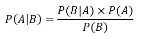
Where:
P(A|B) is the probability that event A occurs given that event B has already occurred.
P(B|A) is the probability that B occurs given that A has occurred. In other words, the opposite probability.
P(A) is the probability of event A occurring and P(B) corresponds to the probability of event B occurring.
In this expression, you should consider the following:

The probability of A given B is not the same as the probability of B given A.
Let’s continue with the previous example.
The probability of contracting the flu (event A) given that we got wet beforehand (event B) could be very high, for example, 80%. A very common scenario in daily life. This is the probability of A given B, P(A|B).
However, the probability of getting wet in the rain (event B) given that we were already sick (A) would be very low, for example, 1%. Imagine this scene: being sick with the flu and getting wet in the rain would be somewhat reckless for a normal person.
Another point to consider is the following: if we observe the equation, we realize that by calculating the opposite conditional probability, that is, P(B|A) and the probabilities of the individual events, P(A) and P(B), we can determine the probability of A given B, P(A|B).
In the day-to-day operations of testing and calibration laboratories or clinical laboratories, determining these probabilities is not as straightforward as solving a typical analytical chemistry exercise.
To solve the equation, we must approach it using Bayes’ theorem in which we estimate values such as sensitivity and specificity, which in turn are estimated by knowing the values of true positives, false negatives, false positives, and true negatives.
If this is the first time you are hearing these terms or are not clear what they mean, don’t worry. In the next section, we will cover them all and provide you with what you need to apply them in the Bayesian approach.
Fundamentals of the Bayes method.

What is a Qualitative Measure?
A qualitative measure is a procedure that yields a result that can be categorized into two or more groups.
If the result is grouped into two categories, it is called a dichotomous result, such as: pass or fail, presence or absence, and positive or negative.
There are other types of tests where qualitative results can be grouped into more than two categories. Some examples of these results include: identifying blood type by observing a binding reagent.
Types of Results in Qualitative Measures.
In addition to the classification of results given in the previous section, we can also classify them based on their truthfulness.
Taking this aspect into account, the values provided in qualitative analysis can be of four types: true positives, true negatives, false positives, and false negatives.
We will explain them briefly, as the Bayes method is based on these concepts:
True Positive (TP).
This occurs when a result provides a positive value for an element that actually possesses the characteristic or analyte of interest.
For example, in a microbiological analysis of Salmonella, a positive result is provided when it was previously known that the analyzed sample contained the bacteria.
False Negative (FN).
This occurs when the result provides a negative value when in reality the analyzed element does possess the characteristic, substance, or analyte of interest.
Example: a urine sample is analyzed to determine the content of alkaloid substances. The result shows a negative value, but in reality, it is positive, given that the sample does contain the alkaloid substance.
True Negative (TN).
It happens when the result of a test provides a negative value when the test item actually does not possess the property or substance to be identified.
Example: A pregnancy test that correctly identifies a sample as negative for the presence of the hCG hormone, indicating that the person is not pregnant.
False Positive (FP).
Occurs when the test value is positive when in reality the result should be negative.
Example: A COVID-19 detection test that mistakenly identifies a sample as positive for the virus when the person is not infected.
Approaches to Estimating Uncertainty in Qualitative Measures Using the Bayes Method.

To estimate the measurement uncertainty in qualitative methods within the laboratory, we can use one of the approaches of the Bayes method.
Each of these approaches is embedded within the same general process and depends on the information available about the test method used.
Based on this, we will deal with 2 approaches to estimating uncertainty in qualitative measurements using the Bayes method.
Approach No. 1 for estimating uncertainty: calculation of sensitivity and specificity.
Imagine that you are in charge of a laboratory and have developed a new analysis method to identify the active ingredient of a drug, such as acetaminophen.
When developing a new method, it is necessary to validate it and therefore estimate its uncertainty. To do this, let’s consider the following scenario:
Suppose we have 100 samples that we previously know contain the active ingredient and 100 samples that do not.
Now, let’s focus on the samples that contain the active ingredient. After analyzing this group of samples using your test method, you obtain the following results: 98 positive results and 2 negative results.
In this case, we obtain 98 true positive results and 2 false negative results. When we relate these two types of results in the same expression, we obtain the sensitivity value of the method, which can be expressed as:
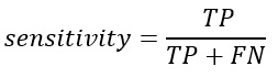
Where TP represents the true positives and FN the false negatives.
For our example, we would have TP equals 98 and FN equals 2, therefore, our sensitivity would be:

If we express it in percentage terms, we have a sensitivity of 98%. That is, out of the 100 samples that we know beforehand contain the active ingredient, our developed method was able to identify 98 samples.
This qualitative method’s capability is known as sensitivity.
Now, focus on the 100 samples that we know do NOT contain the active ingredient. Suppose that after using your method on these 100 samples, the following results were obtained: 95 negative results and 5 positive results.
In this case, we have 95 true negative cases and 5 false positive cases. When we relate these values in the same expression, we obtain the specificity ratio, which is given by:
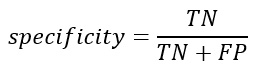
Where TN corresponds to true negatives and FP to false positives. In our example, we have TN equals 95 and FP equals 5, therefore:
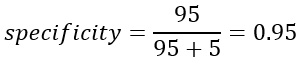
Expressed in percentage terms, this provides us with a specificity of 95%. That is, our method has the ability to identify negative values 95% of the time.
These values of sensitivity and specificity are known as performance parameters of a qualitative method. They are terms originating from clinical sciences.
You should not confuse them with the term analytical sensitivity, as this term is applicable to quantitative analyses.
The values of sensitivity and specificity of a qualitative method are one of the primary approaches when estimating and expressing measurement uncertainty. They are also known by the names of true positive rates, in the case of sensitivity, or true negative rates, for specificity.
Approach No. 2 for Estimating Uncertainty: Calculation of Likelihood Ratios.
This may be one of the most commonly used approaches to estimating uncertainty in qualitative methods.
To do this, we must make use of the concepts of sensitivity and specificity that we have already seen.
There is a likelihood ratio for both positive and negative results, observe it below:
Positive Likelihood Ratio, LR (+).
If we report a positive value, the likelihood ratio is positive and is expressed as follows:
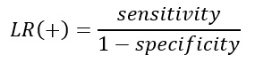
As you can see, these relationships are estimated based on the concepts of sensitivity and specificity that we have already seen.
Interpretation of the Positive Likelihood Ratio LR (+).
Take a break and a good cup of coffee because what’s coming requires your full concentration.
In the positive likelihood ratio, we are comparing two conditional probabilities.
First conditional probability (the one in the numerator of the LR (+) expression): the probability of obtaining a positive result when the case is actually positive.
Second conditional probability (the one in the denominator of the LR (+) expression): the probability of obtaining a positive result when the case is actually negative.
If we take the first conditional probability and divide it by the second, we get the positive likelihood ratio.
If the value of LR (+) is very large, say 1 million, for example, we can be sure that the result is truly positive. Conversely, if the result of LR (+) is negative, the result is not actually positive.
In other words, the likelihood ratio is an indicator of the degree of certainty when reporting a positive result; the higher it is, the greater the reliability that the positive result is true.
Negative Likelihood Ratio LR (-).
On the other hand, the negative likelihood ratio is used when reporting a negative result, and it is calculated as follows:
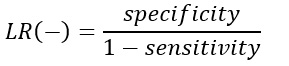
In this case, the negative likelihood ratio compares the following probabilities:
Conditional probability in the numerator: probability that the result is negative given that the item does not contain the property or substance of interest. This value is equal to the specificity of the test method.
Conditional probability in the denominator: probability that the result is negative given that the item of interest does contain the property or substance of interest.
In this case, as the LR (-) increases, there is greater confidence in asserting that the negative result is truly negative and therefore ensuring that the analyzed item does not contain the analyte or property of interest.
In conclusion
Bayes’ Theorem shows us that this old mathematical friend is more useful than we might think, especially when it comes to maximizing the potential of qualitative methods in the laboratory.
By implementing this theorem, we not only enhance the accuracy of our results but also align ourselves with top-quality standards such as ISO/IEC 17025 or ISO 15189.
And yes, it may sound a bit intimidating at first, but once you dive into it, you’ll discover that it’s not as complicated as it seems. So why not continue exploring and applying these good laboratory practices? I promise it will be an exciting journey that is definitely worth it!